Discrete fourier transforms for images
For a few years I’ve put off understanding the fourier transform. I was first introduced to it during an internship at Starlink where I worked on the embedded software team for the satellite phased arrays. To be honest, my understanding was limited to “sin wave -> frequency histogram”. The RF engineers would tell me what band to look for and if my calibration procedure signaled the right one on the readout I was good to go. My days were so frantic that studying the underlying math behind phased arrays wasn’t a priority. Over the years it’s popped up here and there - visiting a friend’s photonics lab, learning about audio signal processing, or trying to intuit H264 compression. Now that I have some freedom to work on and learn broadly, I decided it was time to experiment with it in earnest.
In the rest of this post, my goal is to demonstrate how the discrete fourier transform is helpful in computer vision tasks such as compression and template matching. We’ll build an intuition for 2D sinusoids, implement the discretized fourier transform algorithm, and show some potential applications!
CODE + DATA: https://github.com/aapatni/public in the dft/ folder
Waves can be images too
Let’s start by defining our image $l[n,m]$, with $n$ representing the row indices, and $m$ the column indices.
In 2D the sine and cosine waves can be represented by the functions:
$$s_{u,v}[n,m] = A \sin(2\pi(\frac{un}{N} + \frac{vm}{M}))$$$$c_{u,v}[n,m] = A \cos(2\pi(\frac{un}{N} + \frac{vm}{M}))$$- $u$, $v$ modulate the frequency in the rows and columns
- $A$ is the amplitude of the wave
- $N$, $M$ represent the number of rows, columns in the image
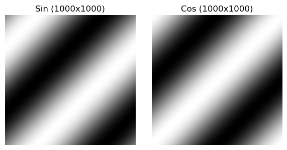
A simple sine and cosine wave may look like:
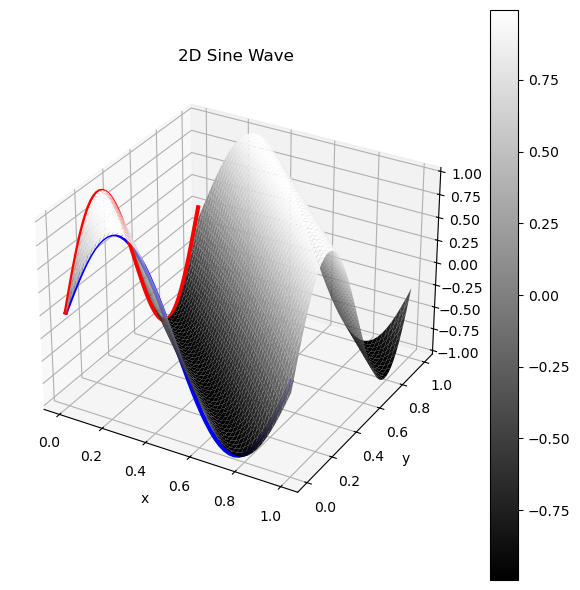
I personally had a hard time understanding the intuition for the above images, so I created a 3D visualization, where the Z axis represents the value of the pixel. This surface when flattened is exactly the same as the sinusoid above! In blue/red I’ve highlighted the 0th column/row of the image, and you can see they trace a sin wave with their amplitudes! The values in between them on the surface are the sine values of their phases combined.
Modulating the spatial frequencies $u,v$
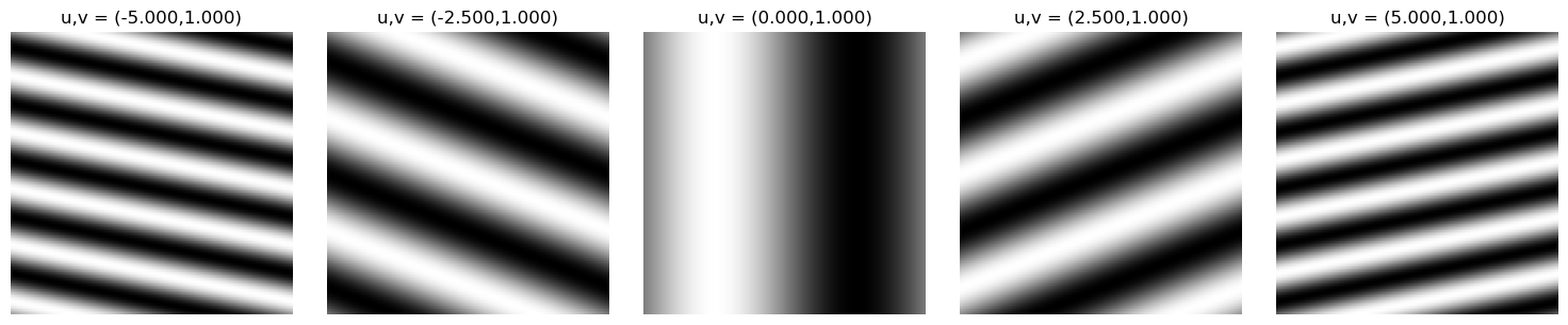
Given our 2D sine image, we can mess around with our parameters $u,v$ to understand how adjusting the spatial frequency changes the appearance of our image. It can stretch, squeeze, and rotate the wave!
Modulating $u$ linearly:
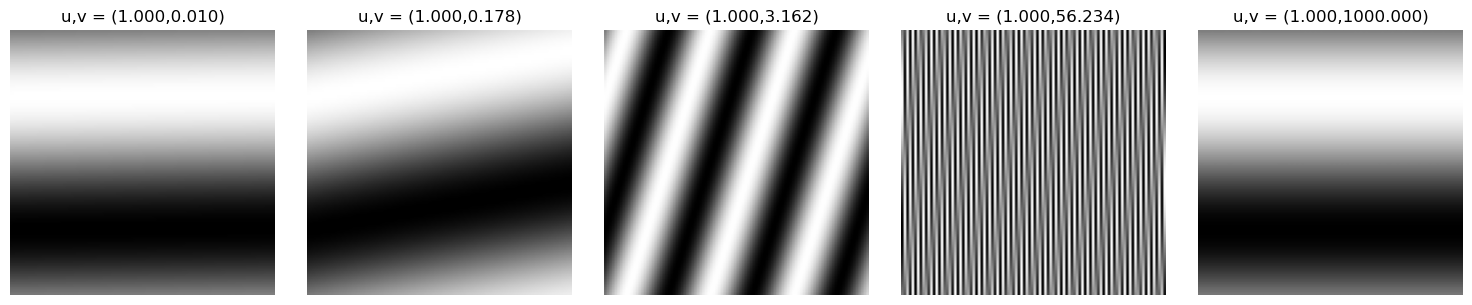
Modulating $v$ exponentially:
The Discrete Fourier Transform (DFT)
The DFT helps us decompose any discrete signal into a sum of complex exponentials (sinusoids). These complex exponentials define a basis for our space, and for any discrete signal, there exists a linear combination of the complex exponential basis functions that can perfectly describe it. The discrete fourier transform relies on this, so understanding this is critical to move forward.
Let’s begin with Euler’s identity, which connects trigonometric functions with complex exponentials:
$$ e^{j\theta} = \cos(\theta) + j\sin(\theta) $$Given an image $l[n,m]$, of size N×M, we can define the basis function:
$$ e_{u,v}[n,m] = e^{2\pi j(\frac{un}{N}+\frac{vm}{M})}$$This represents a 2D complex sinusoid at spatial frequency $(u,v)$. Any discrete image can be decomposed as a linear combination of these. In this formula, the $2\pi$ scales each of our axis to radians (on the unit circle) and the $(\frac{un}{N}+\frac{vm}{M})$ tells us how far into each dimension of the discrete image we are.
We will not prove that the basis functions are orthogonal, but it is possible via the following:
$$\langle e_{u,v}, e_{u',v'} \rangle = 0 \quad \forall (u\neq u'),(v\neq v') $$DFT formula:
Let $L[u,v]$ be the Fourier transform of our image $l[n,m]$, and $F$ be the Fourier transform operator.
$$L[u,v] = F(l[n,m])$$$$L[u,v] = \sum_{n=0}^{N-1} \sum_{m=0}^{M-1} l[n,m]e^{-2\pi j (\frac{un}{N}+\frac{vm}{M})}$$Each coefficient in $L[u,v]$ represents the contribution of a 2D sinusoidal pattern at spatial frequency $(u,v)$. Each term is computed by the inner product between the image and the basis function $e_{u,v}[n,m]$, which intuitively tells us how much of each particular frequency exists in the image.
The DFT decomposes the image into a weighted sum of these frequency components, separating geometry (phase) from energy/brightness (magnitude).
- $∣L[u,v]∣$ is the magnitude spectrum: how much of the frequency exists
- $\arg{(L[u,v])}$ is the phase spectrum: this is the spatial offset of the sinusoid
Note: arg() is the complex equivalent to arctan2(y,x)
Image
Matrix Form:
$$ \begin{bmatrix} 4.0+0.0j & -3.8-1.4j & \cdots & 3.0+2.5j \\ 2.2-1.9j & 1.4+2.5j & \cdots & -2.9+0.0j \\ \vdots & \vdots & \ddots & \vdots \\ -2.2+1.9j & 2.7+1.0j & \cdots & -0.5+2.8j \end{bmatrix} $$Inverse formula:
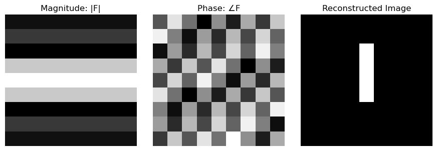
$$l[n,m] = F^{-1}(L[u,v])$$$$l[n,m] = \frac{1}{NM} \sum_{u=0}^{N-1} \sum_{v=0}^{M-1} L[u,v]e^{+2\pi j (\frac{un}{N}+\frac{vm}{M})}$$The inverse DFT reconstructs the image as a weighted sum of complex sinusoids. Each term contributes a wave pattern whose amplitude is $∣L[u,v]∣$ and shift is determined by $\arg{(L[u,v])}$.
Computing the DFT
Below I will lay out the code for the discrete fourier transform (and it’s inverse). Computing the DFT in this way is extremely computationally inefficient, and there are much faster ways to compute the discrete fourier transform. In future examples I will use numpy’s fft2() functions to perform this operation in $O(N^2log(N))$ time complexity instead of $O(N^4)$.
def compute_fourier_tfm_slow(image: np.ndarray) -> np.ndarray:
    N,M = image.shape
    output = np.zeros((N,M), dtype=complex)
    for u in range(N):
        for v in range(M):
            for n in range(N):
                for m in range(M):
                    output[u,v] += image[n,m] * np.exp(-2j*np.pi*((u*n/N)+(v*m/M)))
    return output

def compute_inverse_fourier_tfm_slow(fourier_image:np.ndarray) -> np.ndarray:
    N,M = fourier_image.shape
    output = np.zeros((N,M), dtype=complex)
    for n in range(N):
        for m in range(M):
            for u in range(N):
                for v in range(M):
                    output[n,m] += fourier_image[u,v]*np.exp(2j*np.pi*((u*n/N)+(v*m/M)))
    output *= 1/(N*M)
    return output
Visualizing the Fourier Matrix
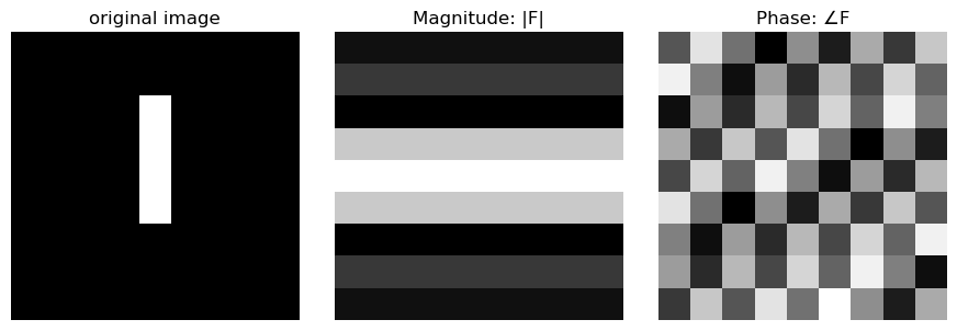
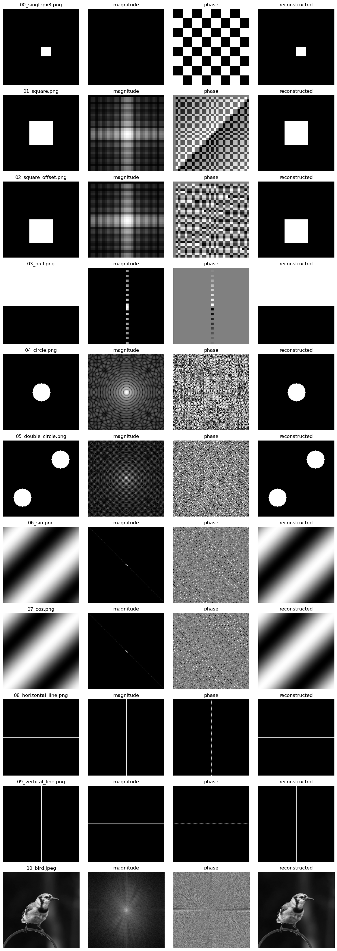
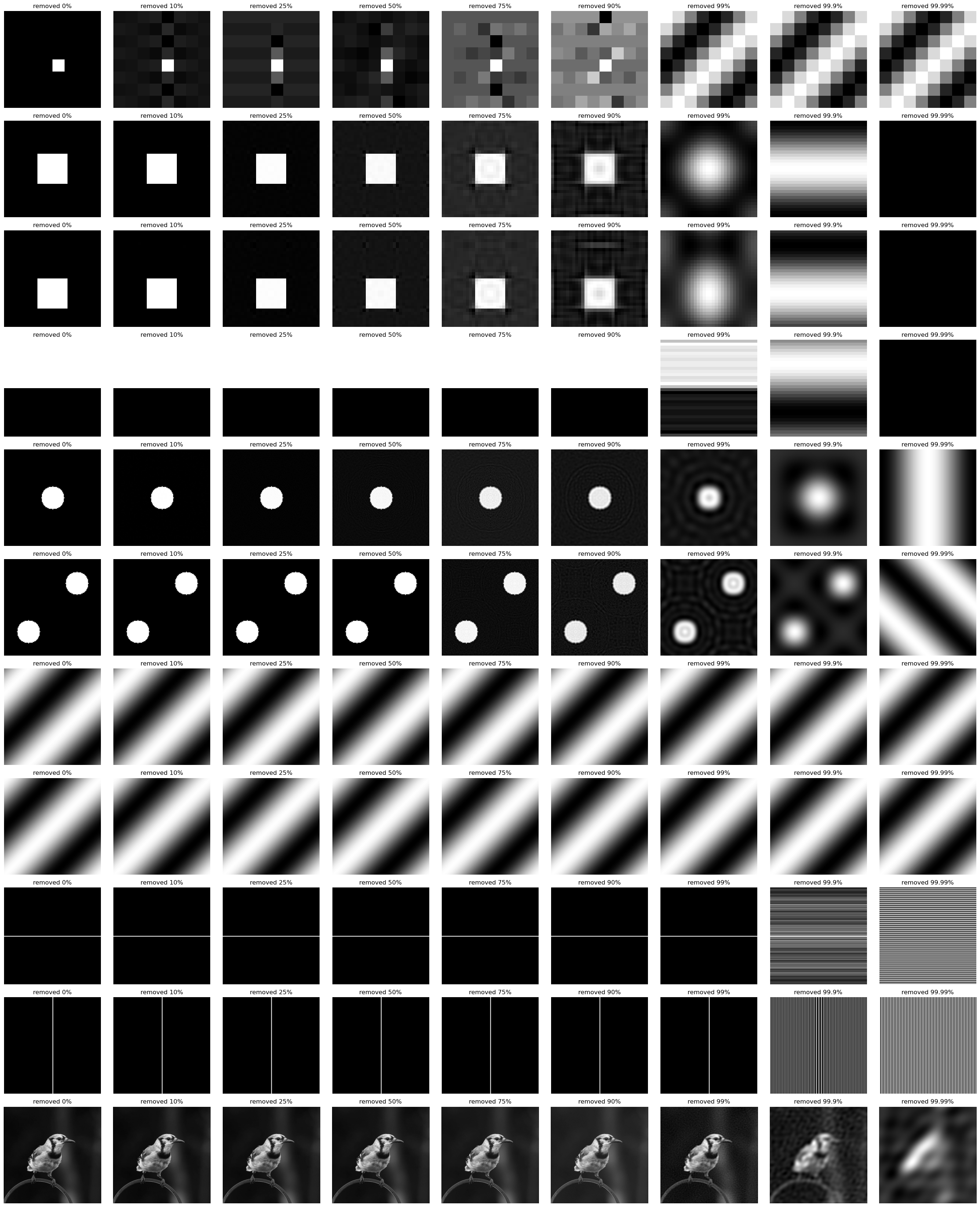
When visualizing the fourier matrix, we must decompose it into a phase and magnitude image because each term is a complex number. In making these visualizations I performed some extra modifications to the matrix to make it slightly more interpretable (you can view the code in the attached notebook). This amounts to centering the low frequency components in the matrix, and shifting higher frequency components to the edges.
I find these visualizations quite beautiful, and I recommend you take a few minutes to inspect each image and it’s corresponding phase / magnitude.
How is this used in the real world?
In the next section we’ll go over uses for the discrete fourier transform in image analysis. The primary ones I know about are compression and image registration/alignment.
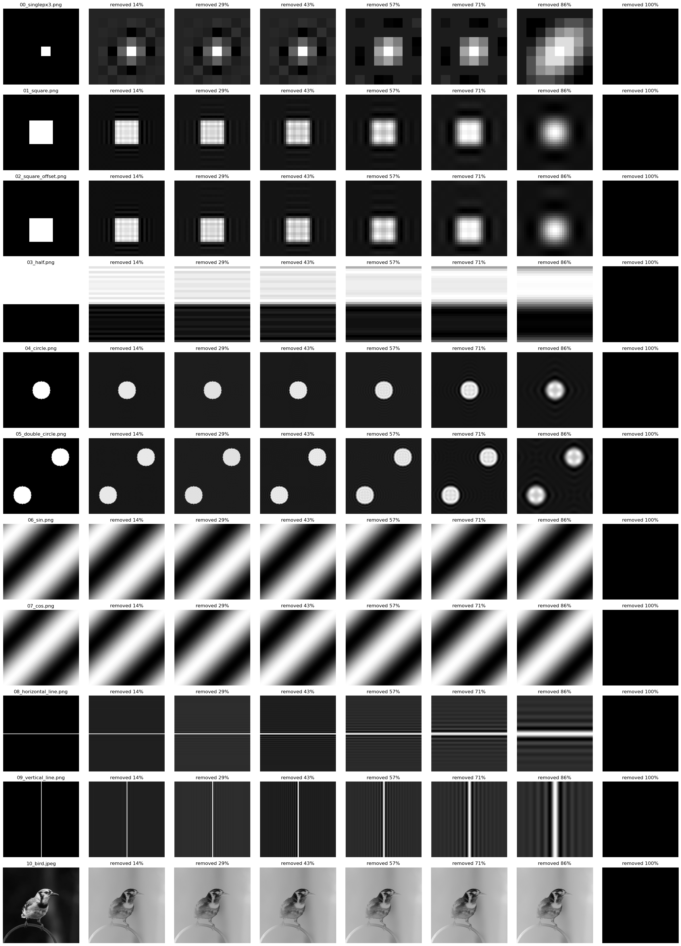
Compression: removing high frequency terms
Removing the high frequency terms from the fourier matrix can be used to compress an image. As more and more of these terms are zeroed out, you will notice that the features in the image will blur, because the finer grained edges can’t be represented by the lower frequency complex exponentials.
Notice that sin/cos patterns survive this form of compression because they are represented by only the lowest frequency components of the fourier matrix.
Method:
- Perform the fourier transform on an input image
- Set X% of high frequency terms to 0
- Perform the inverse fourier transform
- Visualize
Compression: removing low magnitude factors
Next, we’ll try a similar technique, but instead zero out factors that are lower magnitude $|F[u,v]|$.
Method:
- Perform the fourier transform on an input image
- Set X% of lowest magnitude terms to 0
- Perform the inverse fourier transform
- Visualize
Compression: towards JPEG
While implementing the above compression methods, I learned that JPEG compression is based on similar frequency-domain principles. At a high level, JPEG divides the image into 8×8 blocks, applies a frequency transform, and then quantizes the resulting coefficients to achieve compression.
JPEG specifically uses the Discrete Cosine Transform (DCT) rather than the DFT. The DCT uses only real-valued cosine basis functions, which makes it more efficient storage and computation. There are many differences between the JPEG spec and the method I’ve laid out below, so do check out an external resource on JPEG for the exact spec.
Method:
- Block-wise Decomposition: Chunk the image into 8x8 sections
- Fourier Transform: Apply the fourier transform to this chunk and perform an
fft_shift()to center the high frequency domains - Quantization: Element-wise apply the quantization matrix (see in code)
- low-frequency components (closer to the center of the block [4,4]) should be preserved more than high frequency components
- tunable scale parameter $Q[i,j] = Q[i,j]^{scale}$ controls the compression aggressiveness. The range for my scale parameter is [0,$\inf$], unlike most typical scaling parameters [0,100].
- Sparsification: Set all coefficients with magnitude < 1.0 to 0 to sparsify the fourier matrix
- Storage: Convert the result to Compressed Sparse Row (CSR) format to reduce memory usage, exploiting the sparsity introduced by quantization.
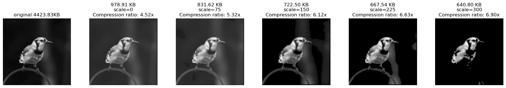
On a real image this works quite well!
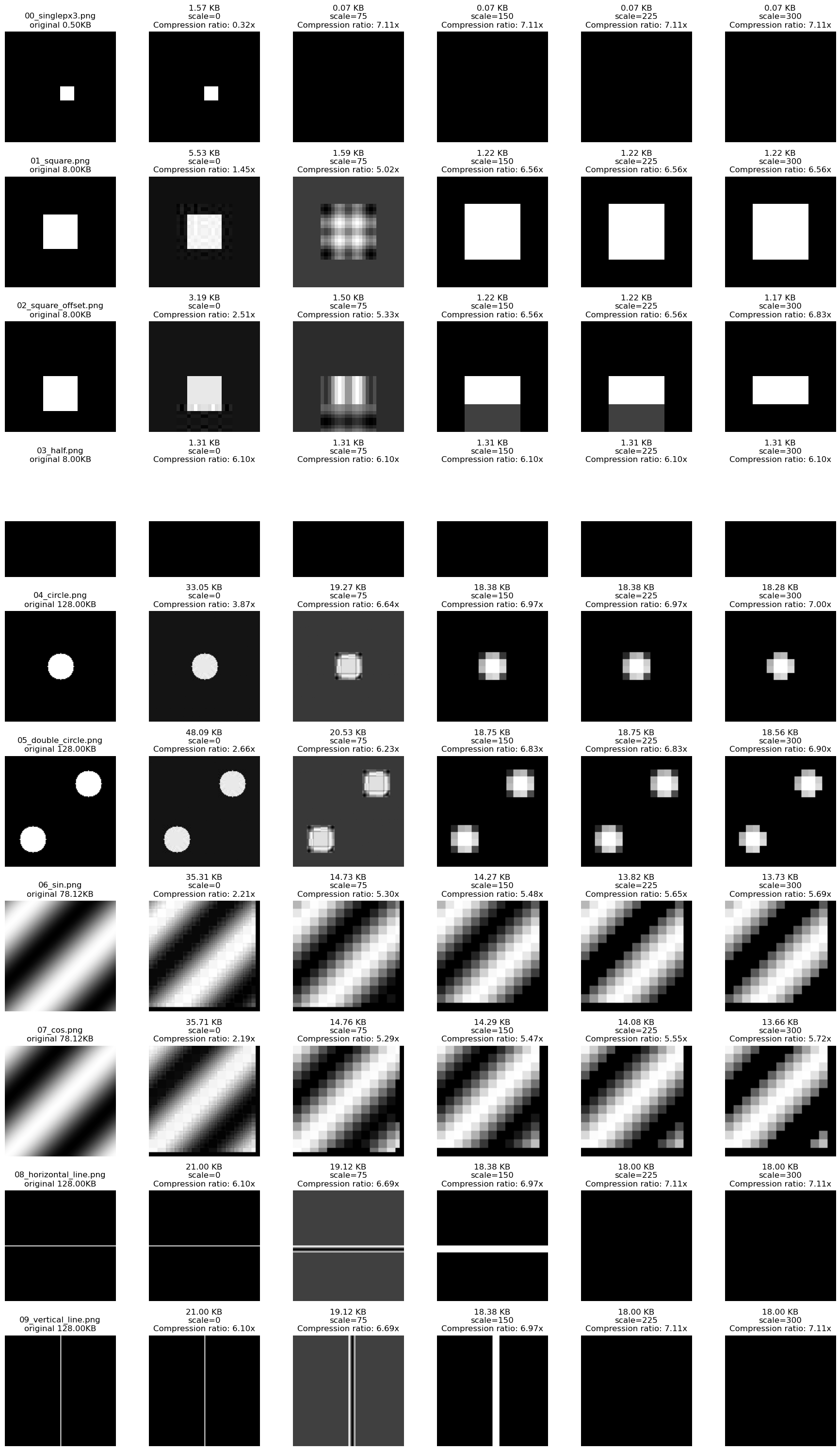
On the simple test images I manually generated, this 8x8 chunking performs poorly.
Template Matching
Another use case for the fourier transform is in a very basic task: template matching.
What is template matching?
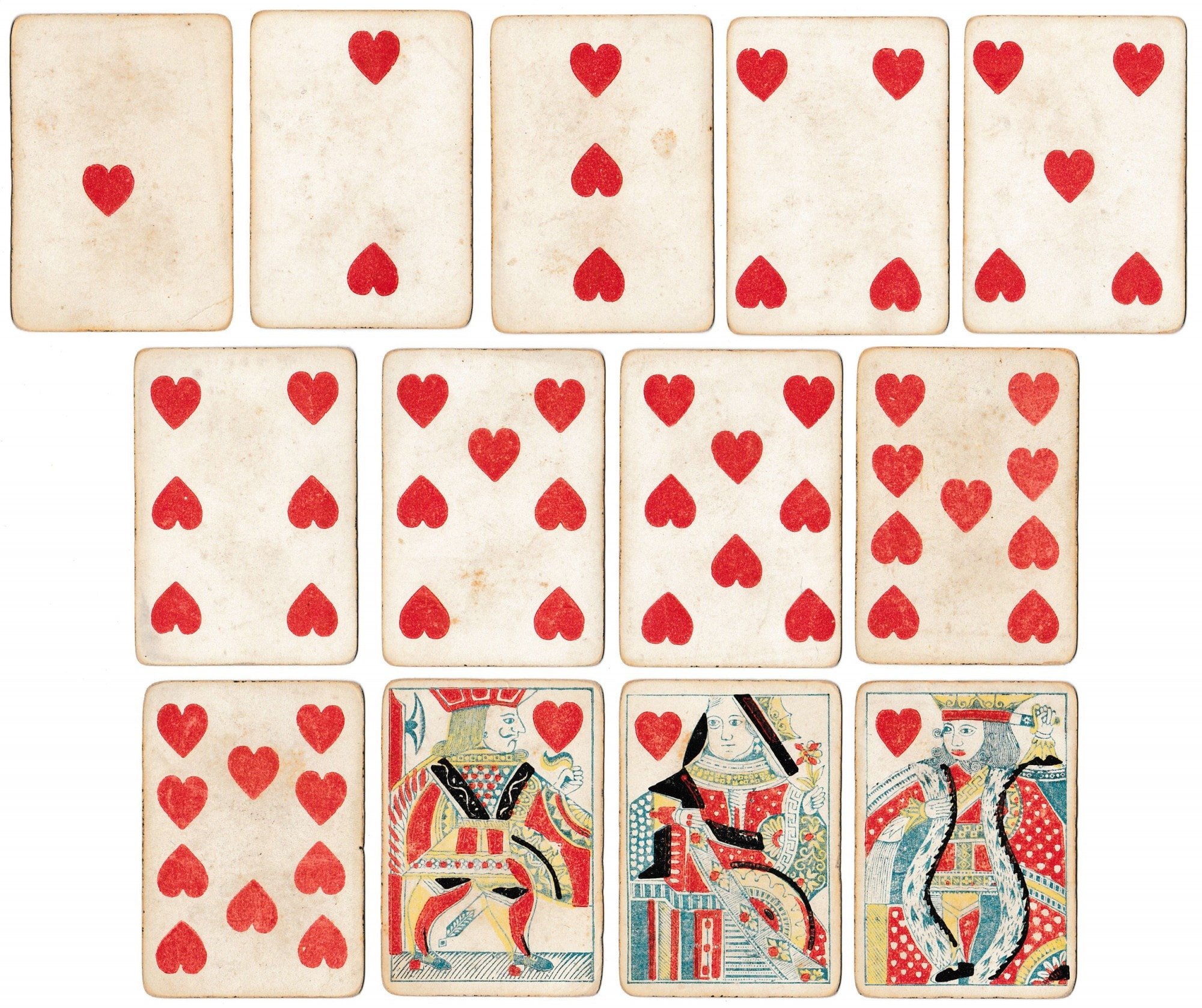
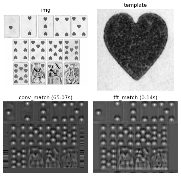
Given an input image (I) and a template (T), can we find all instances of T in I?

Template matching is often computationally expensive because we need to compute the cross-correlation between a template $T$ and an image $I$ at every possible spatial offset - essentially sliding the template over the image and measuring the similarity at each location. This produces an output map $C$ where high values indicate strong matches.
Fortunately, due to the Convolution Theorem, we can compute this more efficiently in the frequency domain. Cross-correlation can be computed by applying the fourier transform to both $I$ and $T$, multiplying $F(I)$ with the complex conjugate of $F(T)$, and applying the inverse fourier transform to get back to the spatial domain. The result is a correlation map where high values correspond to locations where the template matches the image.
Imagine we want to convolve the function $f(t)$ and $g(t)$ to measure the similarity between $f$ and $g$ at each possible offset. The convolution theorem connects our abilities to do this timestep by timestep with the ability to check this in the frequency domain.
Convolution Theorem:
$$\begin{align} \underbrace{f(t)\circledast g(t)}_{\text{convolution}} &= \underbrace{F^{-1}}_{\text{inverse fourier}}(F(f(t))\cdot F(g(t))) \end{align}$$We can extend this formula to cross correlation across images and template images with the following:
Cross Correlation:
$$\begin{align}\underbrace{C}_{\text{correlation map}} &= F^{-1}(\underbrace{F(I)}_{\text{image}} \cdot \underbrace{\overline{F(T)}}_{\text{conj of template}})\\ \end{align}$$def match_via_convolution(image: np.ndarray, template: np.ndarray) -> np.ndarray:
N,M = image.shape
Nt, Mt = template.shape
template = template - np.mean(template)
template = template / np.max(np.abs(template))
response = np.zeros_like(image)
for i in range(0, N-Nt+1):
for j in range(0,M-Mt+1):
patch = image[i:i+Nt, j:j+Mt]
patch = patch - np.mean(patch)
patch = patch / np.max(np.abs(patch))
response[i,j] = np.sum(patch*template)
response = response - np.mean(response)
response = response / np.max(np.abs(response))
return response
def match_via_fft(image: np.ndarray, template: np.ndarray) -> np.ndarray:
N, M = image.shape
Nt, Mt = template.shape
assert (N>=Nt and M>=Mt), "template should be smaller than image"
template = template - np.mean(template)
template = template / np.max(np.abs(template))
padded_template = np.zeros_like(image)
padded_template[:Nt, :Mt] = template
Ft = np.fft.fft2(padded_template)
Fi = np.fft.fft2(image)
corr = np.real(np.fft.ifft2(Fi * np.conj(Ft)))
corr = corr - np.mean(corr)
corr = corr / np.max(np.abs(corr))
return corr
Cross Correlation Visualization
Using the fast fourier transform for template matching provides a dramatic ~500x speedup compared to direct convolution on a (2k,1k) pixel image!
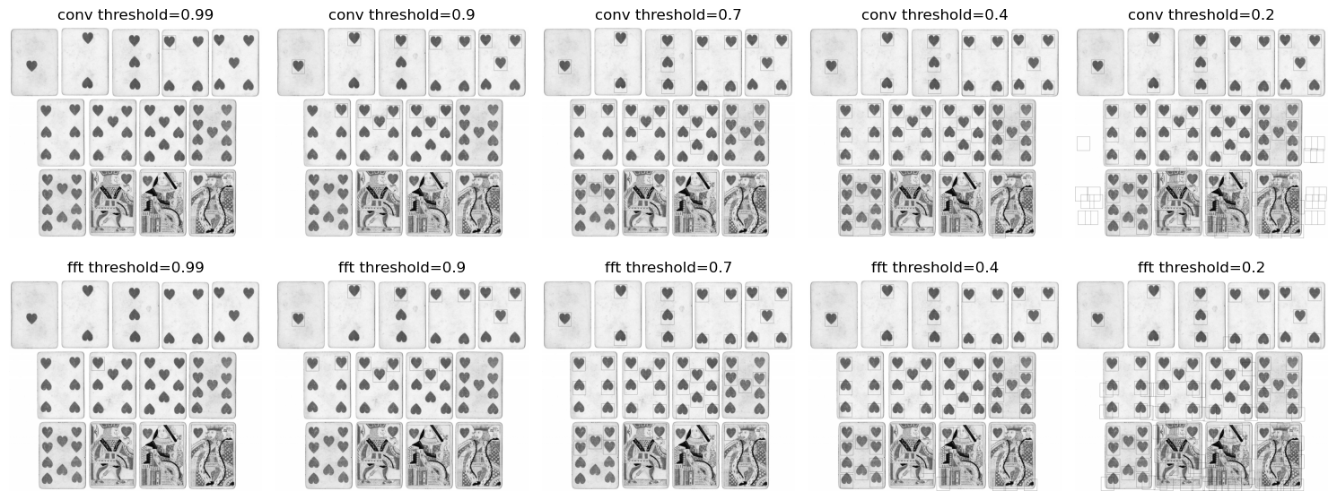
To obtain the final template matches we first threshold the cross correlation image and then perform non maximal suppression on the resulting bounding boxes. Shown below are the bounding boxes drawn on the image at various thresholds. As we lower the threshold, more errors are introduced, like upside down hearts and white patches, which yield higher responses than randomized patches. Also note the similarities and differences between the outputs of the convolutional method and the DFT based method.
Wrapping it up
The fourier transform is pretty useful, beautiful, and computationally efficient for a variety of computer vision tasks. I hope you enjoyed the visualizations! Code + data is located here: https://github.com/aapatni/public in the dft/ folder