After working on the discrete fourier transform, I became interested in how image compression works and, in particular, how vision companies select their quantization (Q) matrices. Today these matrices are often hand-crafted, with the Human Visual System (HVS) used as the yardstick for deciding which candidate preserves perceptual quality.

But in most modern applications, cameras aren’t producing images for humans - they’re producing data for models. That changes the objective: instead of optimizing Q matrices for what the human eye prefers, we could optimize them for two criteria: (1) compressibility, and (2) performance of downstream vision models. This feels like a natural step toward fully end-to-end camera pipelines, where every layer from lens to pixel representation is tuned for a singular objective.

At this point you might ask: why not just use neural compression? Neural codecs are promising, but the practical barrier is hardware. The vast majority of production cameras ship with fixed-function ASICs for JPEG/H.264/H.265, not NPUs capable of running learned codecs. Until silicon support changes, I thought it made more sense to stay within the existing paradigm and push Q-matrix optimization as far as it can go.

JPEG codec overview

It’s important to understand the high level steps in the jpeg codec, for a full review I’d advise you to check out: short, medium or long guide.

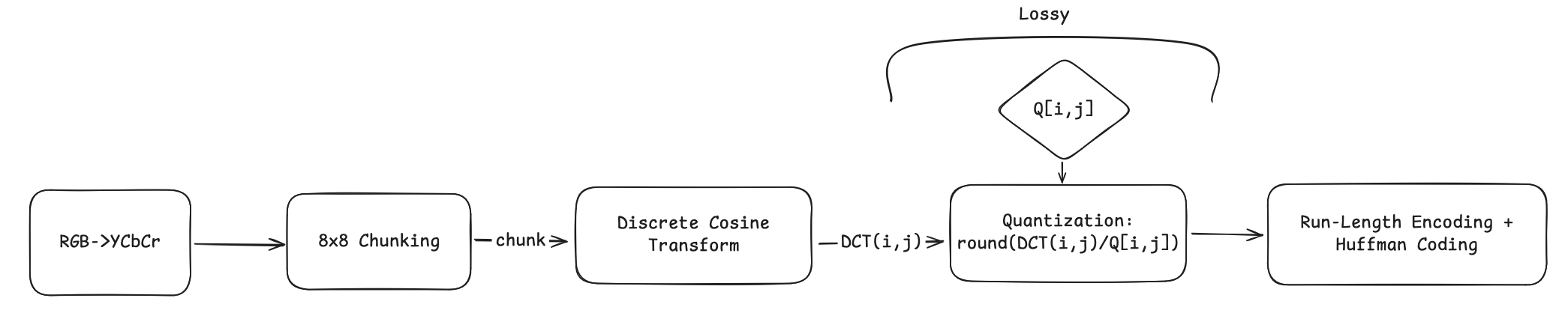
Note: the lossy step is where the magic happens!

Vision Pipeline

At a high level, the vision pipeline looks like this:

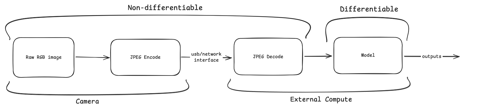
Images are captured, encoded, and then transmitted over a hardware interface to the machine where decoding and inference are performed. Information has already been lost by the time an image reaches the model. JPEG encoding discards detail at the quantization step, and our downstream model can only work with what survives.

The question, then, is how do we maximize model performance (bounding boxes, segmentation, VLM tasks) given that we must compress?

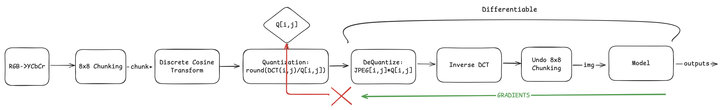
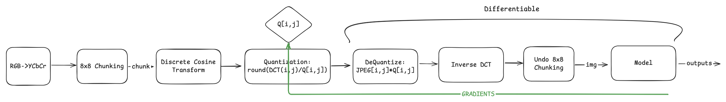
My overarching thesis was that we could be more selective about which coefficients get discarded by directly optimizing the JPEG Q matrix. The search space for this Q is quite large, and so using gradient descent is required - meaning that we need a differentiable path from the model’s loss all the way back through JPEG.

Most of this pipeline is straightforward: color transforms, block splitting, DCT, dequantization, and inverse DCT are all linear or lossless operations. The one roadblock is quantization, where we divide by Q and apply rounding. Standard rounding has zero gradient, which breaks backpropagation.

Fortunately, the lossless steps after quantization don’t affect the gradient path (RLE+Huffman). They help minimize the bit-rate, but are perfectly reconstructed by the decoder. We can drop them during training and only keep what matters for learning Q:

The last step is differentiable rounding. Unfortunately the gradient for torch.round(x) is 0 everywhere. To fix this, we replace it with a surrogate that pulls values toward integers while still passing gradients:

$$ y = \text{round}(x) + (x-\text{round}(x))^3$$

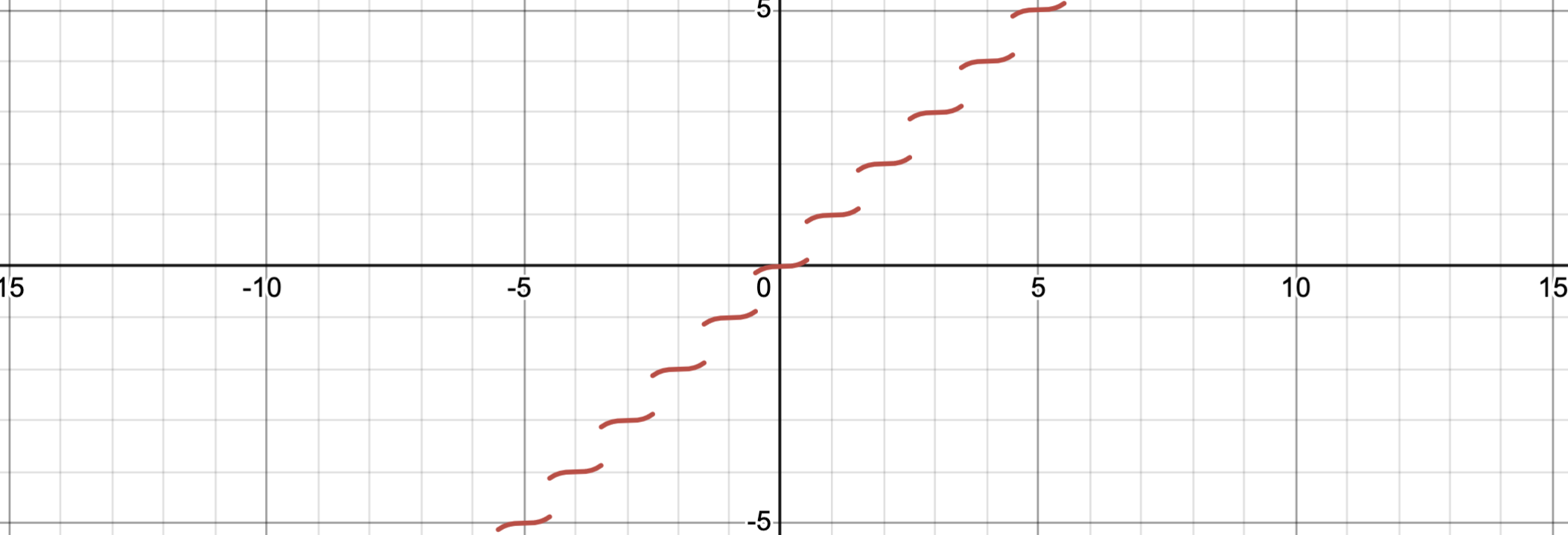
This cubic term shrinks values toward the nearest integer in the forward pass, but its derivative provides a smooth gradient almost everywhere which enables the loss to propagate back towards the Q.

$$ \frac{dy}{dx} = 3(x-\text{round}(x))^2 $$

So now we can push gradients from our unchanged model’s loss function all the way back through to the Q matrix in our new implementation of differentiable jpeg.

Setup

The architecture is relatively simple: differentiable JPEG compression feeds into YOLOv5, with gradients flowing back to update only the quantization matrices while keeping all other parameters frozen. Rather than dive into pytorch implementation details, I’ll list out some of the references that got me started:

• Dataset: https://huggingface.co/datasets/bryanbocao/coco_minitrain/blob/main/coco_minitrain_25k.zip
• Model: https://github.com/ultralytics/yolov5 (task: object detection)
• Differentiable compression library: https://github.com/kornia/kornia

Benchmarking PIL against Kornia

To ensure that Kornia’s implementation (with my modifications) was consistent with PIL’s standard jpeg compression at various quality levels, I performed an test across some images in my validation set.

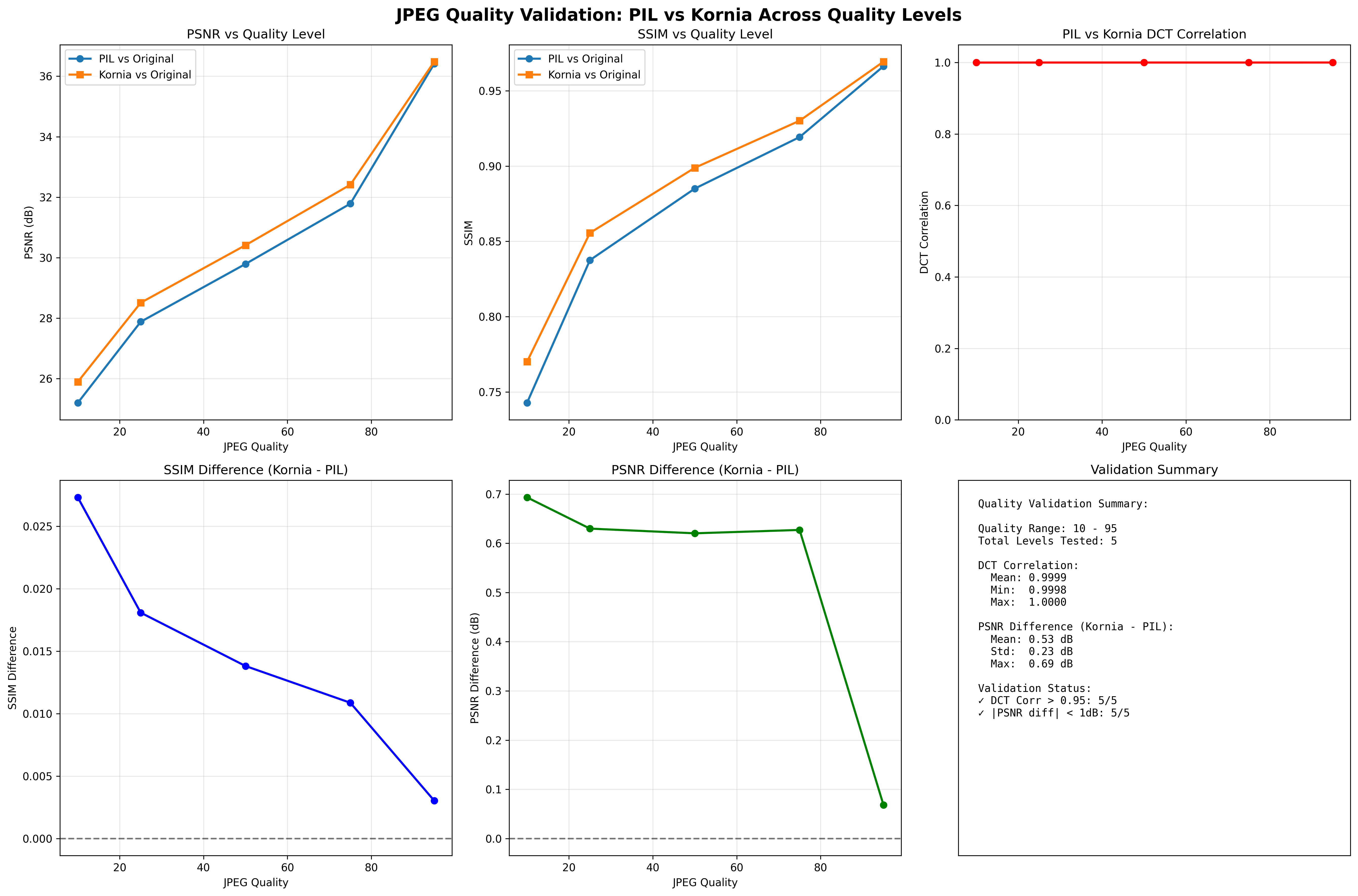
PSNR (peak signal to noise ratio) - represents how closely the signal/ratio across the original matches to the distorted image

SSIM (structural similarity index) - compares textures, edges, and structures in the image

As you can see, Kornia tracks PIL very closely on both metrics, which means we can trust it as a differentiable drop-in replacement for JPEG.

Training / Experiments

Baseline with Default Q

First, I established a baseline by training YOLOv5 with the default JPEG quantization tables (no optimization).

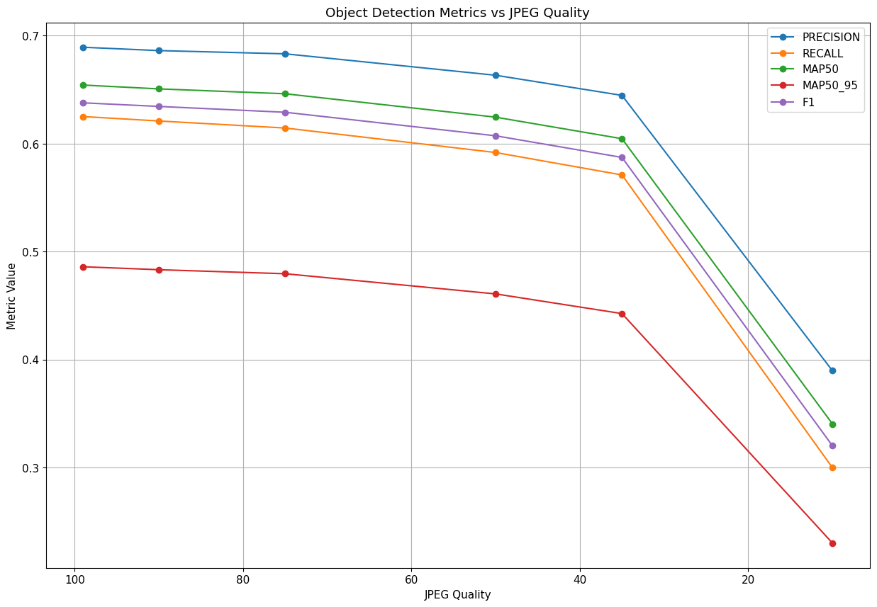
This gives us a reference MAP (mean average precision) performance on the dataset with standard compression.

YOLO only - what could go wrong?

My first experiment was to directly optimize Q matrices using YOLO’s loss function alone. YOLO’s total loss is a weighted sum of three primary components:

1. Localization loss (IoU) — how well the predicted bounding box matches the ground truth.
2. Objectness loss (BCE) — how confident the model is that an object exists in the box.
3. Classification loss (BCE) — how well the model identifies the object’s category.

The idea: let the model’s detection loss guide which image features should survive compression.

Result:

Training diverged. MAP collapsed quickly.

I realized there were a few problems in my training that I modulated around with some small performance boosts (step size too big, poor optimizer/scheduler choices).

More fundamentally, YOLO’s loss alone isn’t expressive enough: it rewards detection but has no penalty for catastrophic visual degradation.

So the network found degenerate Q matrices that helped bounding boxes in the short term but destroyed image quality.

Next Steps:

Integrate reconstruction loss into the loss function so that image quality could be preserved.

Staying Similar: Adding SSIM to Loss

SSIM captures structural fidelity, so it provides a direct penalty when compression distorts edges, textures, or shapes.

The combined loss looked like:

$$L=YOLO+λ(1−SSIM)$$

Result:

SSIM stayed high — images remained perceptually stable.

MAP stopped tanking and detections were usable again.

But upon inspection the Q matrices all started collapsing toward zero.

Why? The model discovered that setting Q=1 skips quantization entirely (perfect reconstruction), which trivially maximizes SSIM and stabilizes MAP. As usual, the network found a shortcut — it learned to bypass compression altogether.

Next Steps:

Include a proxy loss that tries to keep values in the Q matrix high.

Also - my plots weren’t expressive enough - I needed to up my matplotlib game and log more data throughout the training process - things like intermediate Q matrices and metrics around how they’re evolving.

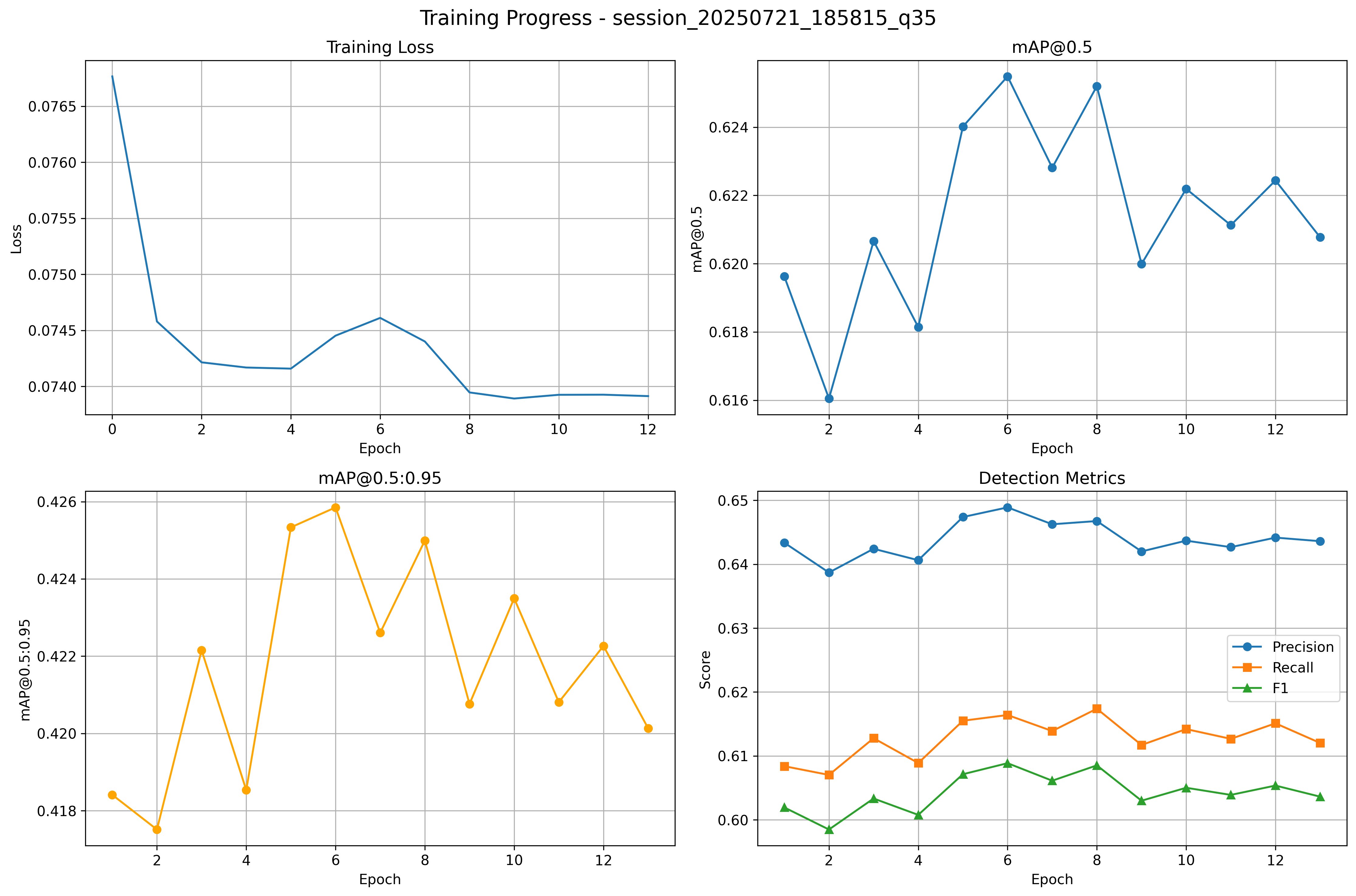
Keep Compressing: Integrating $\overline{Q}$ as a proxy loss

The next direction was to integrate metrics around the compression matrix into the loss function - namely maximizing the mean value of elements in the matrix.

$$L=YOLO+λ_s(1−SSIM)-λ_q\overline{Q}$$

Result:

Compression ratio as a proxy loss

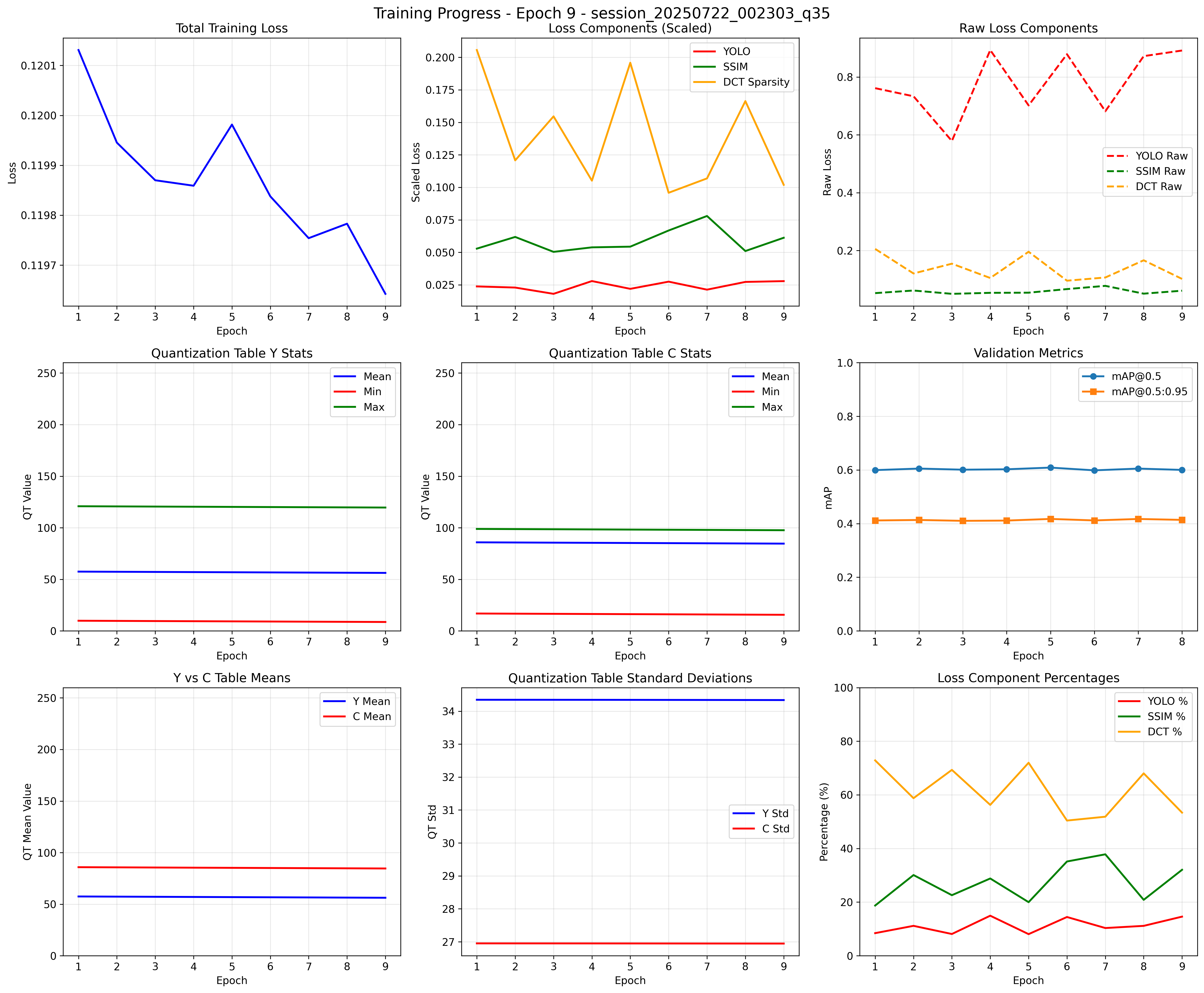
$$L=YOLO+λ_s(1−SSIM)+λ_c(\frac{bytes(Img_o)}{bytes(Img_c)})$$

Unfortunately, using the raw bytes ratio as a loss was unstable. Different images vary a lot in how well they compress, so across minibatches the file sizes are not i.i.d. The result was that the compression loss jumped around too much during SGD. To fix this, I replaced the bytes ratio with a proxy based on sparsity of the quantized DCT coefficients. This is more stable across batches and directly tied to JPEG’s compression mechanism.

$$L=YOLO+λ_s(1−SSIM)+λ_c(\text{Sparsity})$$

Result:

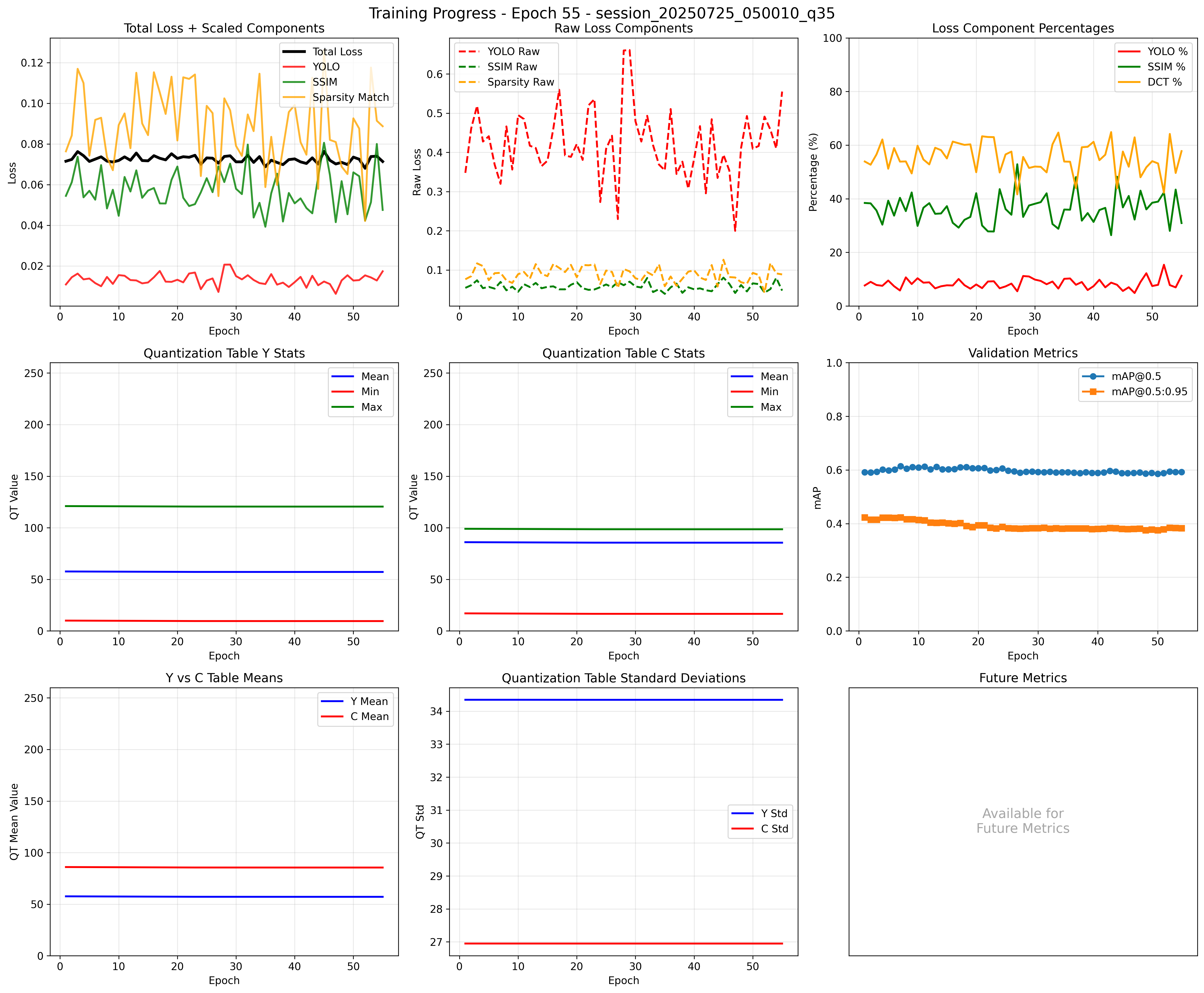
Finally! The quantization table mean values stay consistent over many epochs, but unfortunately this came at the cost of YOLO loss spiking. The compression ratio’s of these new matrices were low, so the proxies that we constructed weren’t effective at keeping the compression ratios stable.

Final State

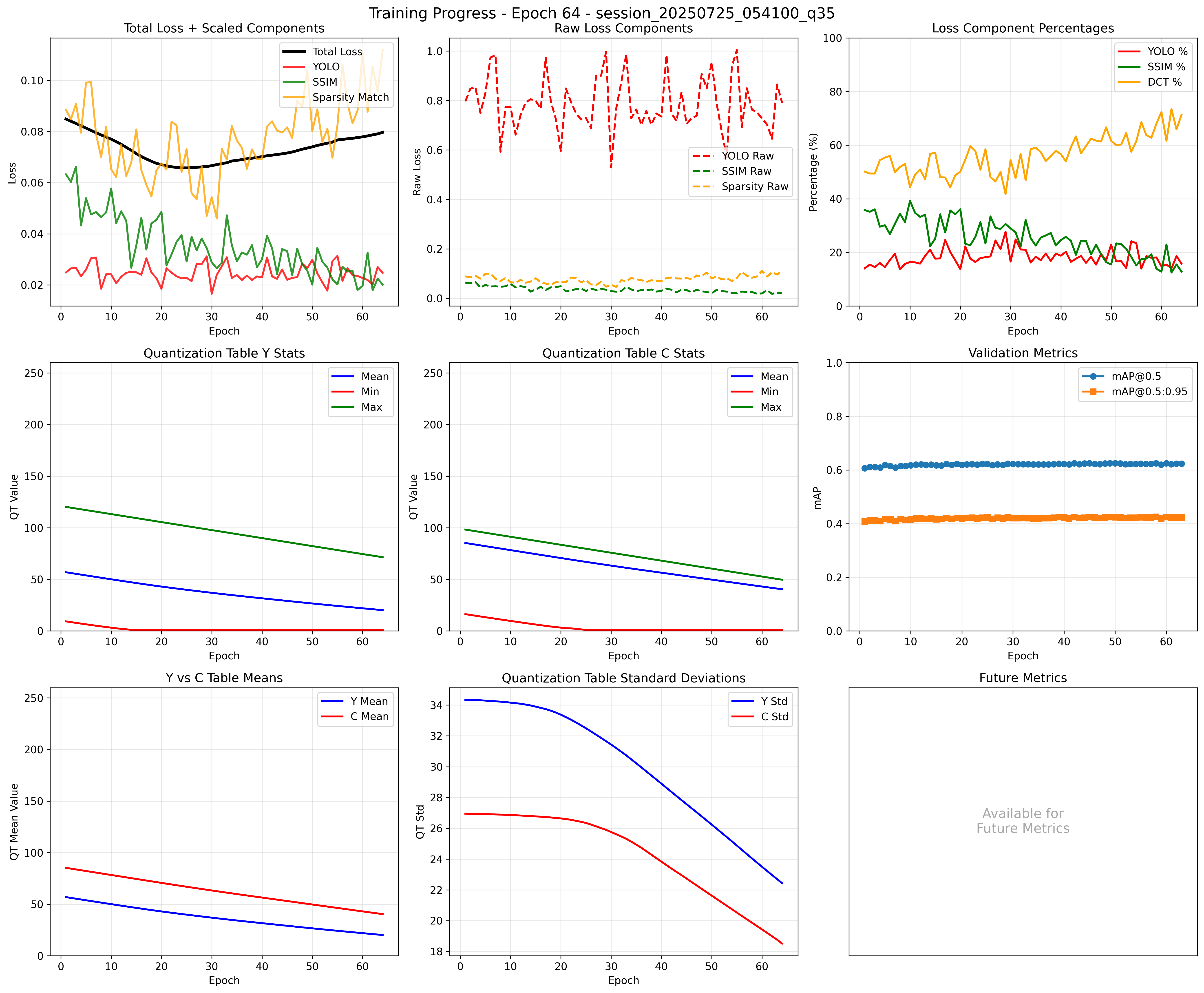
After a lot of fine-tuning and tweaking I reached a relatively unsatisfying end state, the quantization matrices constructed are not simultaneously compressive and performant for YOLO. So, I’ve decided for now to pause on this project and focus on other areas of exploration in robotics. Hopefully in the future I can write a follow up to this project and publish new quantization matrices that help object detection companies around the world.